<?xml version="1.0" encoding="utf-8"?><feed xmlns="http://www.w3.org/2005/Atom" xml:lang="es"><generator uri="https://jekyllrb.com/" version="4.4.1">Jekyll</generator><link href="https://3cucharadas.cl/en/feed/politica-publica.xml" rel="self" type="application/atom+xml" /><link href="https://3cucharadas.cl/en/" rel="alternate" type="text/html" hreflang="es" /><updated>2026-07-05T20:48:44-04:00</updated><id>https://3cucharadas.cl/feed/politica-publica.xml</id><title type="html">3 Cucharadas | Politica-publica</title><subtitle>Explorando curiosidades</subtitle><author><name>Cristián Labra Olivares</name></author><entry xml:lang="en"><title type="html">CASEN 2024 in 3 spoonfuls: without a fine-grained territorial reading, social policy moves blind</title><link href="https://3cucharadas.cl/en/datos/politica-publica/julia/casen/casen2024-julia-waffles-politica-publica/" rel="alternate" type="text/html" title="CASEN 2024 in 3 spoonfuls: without a fine-grained territorial reading, social policy moves blind" /><published>2026-03-15T00:00:00-03:00</published><updated>2026-03-15T00:00:00-03:00</updated><id>https://3cucharadas.cl/datos/politica-publica/julia/casen/casen2024-julia-waffles-politica-publica-en</id><content type="html" xml:base="https://3cucharadas.cl/datos/politica-publica/julia/casen/casen2024-julia-waffles-politica-publica/"><![CDATA[<p>In Chile, <strong>La Araucanía records 13.0% extreme poverty; Magallanes, 4.2%</strong>. That is 8.8 percentage points of difference — and if a public agency at the central or local level (regional governments / municipalities) designs its intervention using only the national average (6.9%), or disregarding regional differences, it could get the allocation of resources or the distribution of its components wrong.</p>

<p>This post documents a reproducible analysis of CASEN 2024 in <a href="https://julialang.org">Julia</a>, with cross-validation of official public figures against BIDAT and good traceability of the flow in the repo.</p>

<p><strong>Three findings to start with — statistically robust:</strong></p>

<ul>
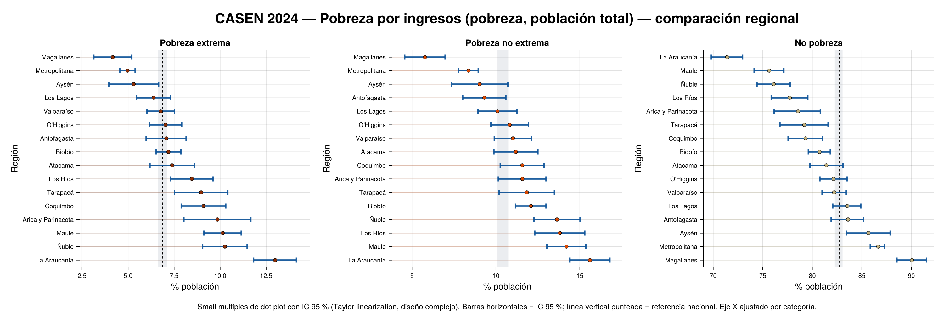
  <li><strong>Extreme poverty</strong>: La Araucanía 13.0% 95% CI [11.8%, 14.1%] versus Magallanes 4.2% [3.1%, 5.2%] — a gap of <strong>8.8 pp with non-overlapping CIs</strong>.</li>
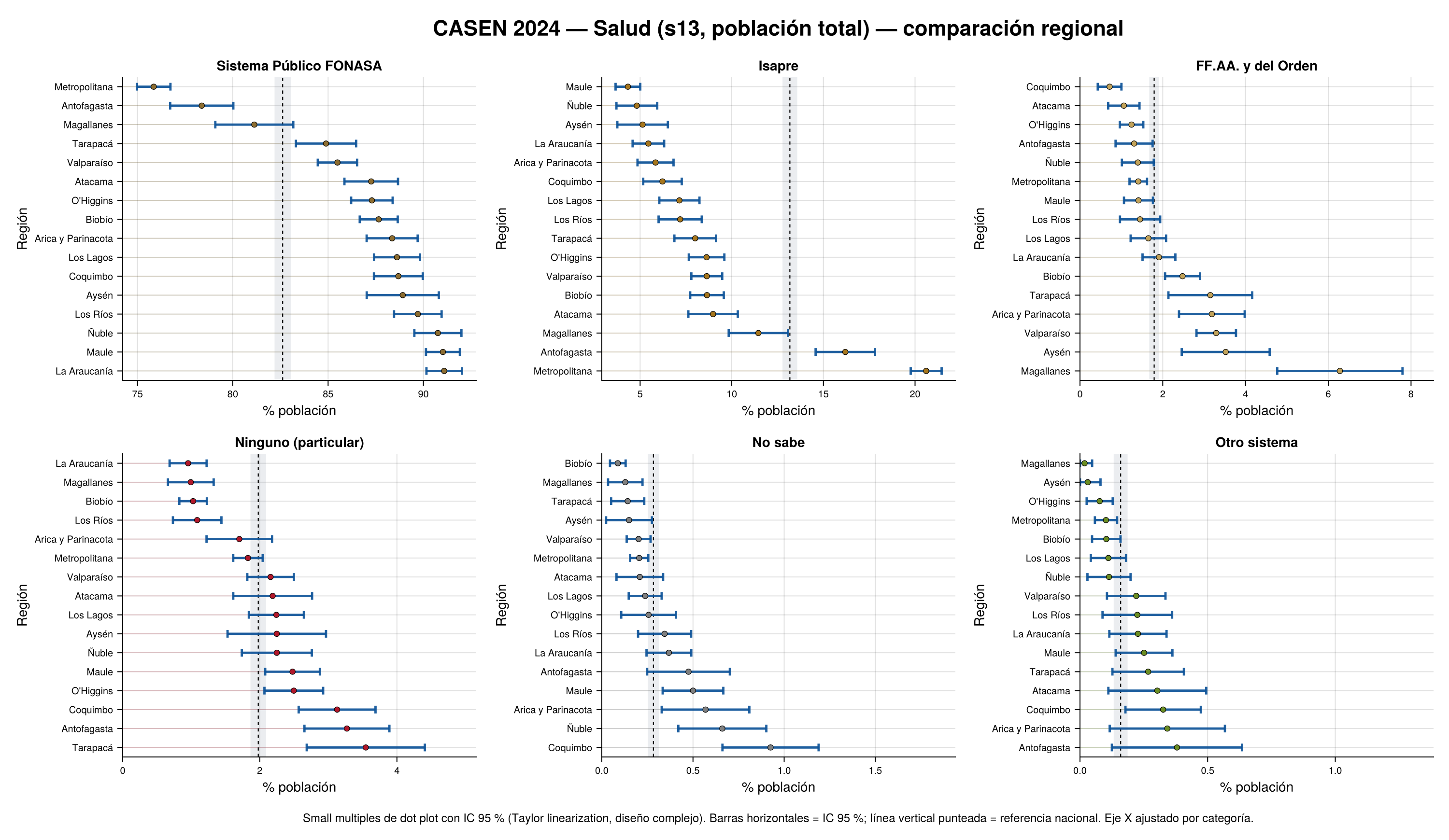
  <li><strong>FONASA coverage</strong>: La Araucanía 91.1% [90.2%, 92.0%] versus Metropolitana 75.9% [75.0%, 76.7%] — a gap of <strong>15.2 pp with non-overlapping CIs</strong>.</li>
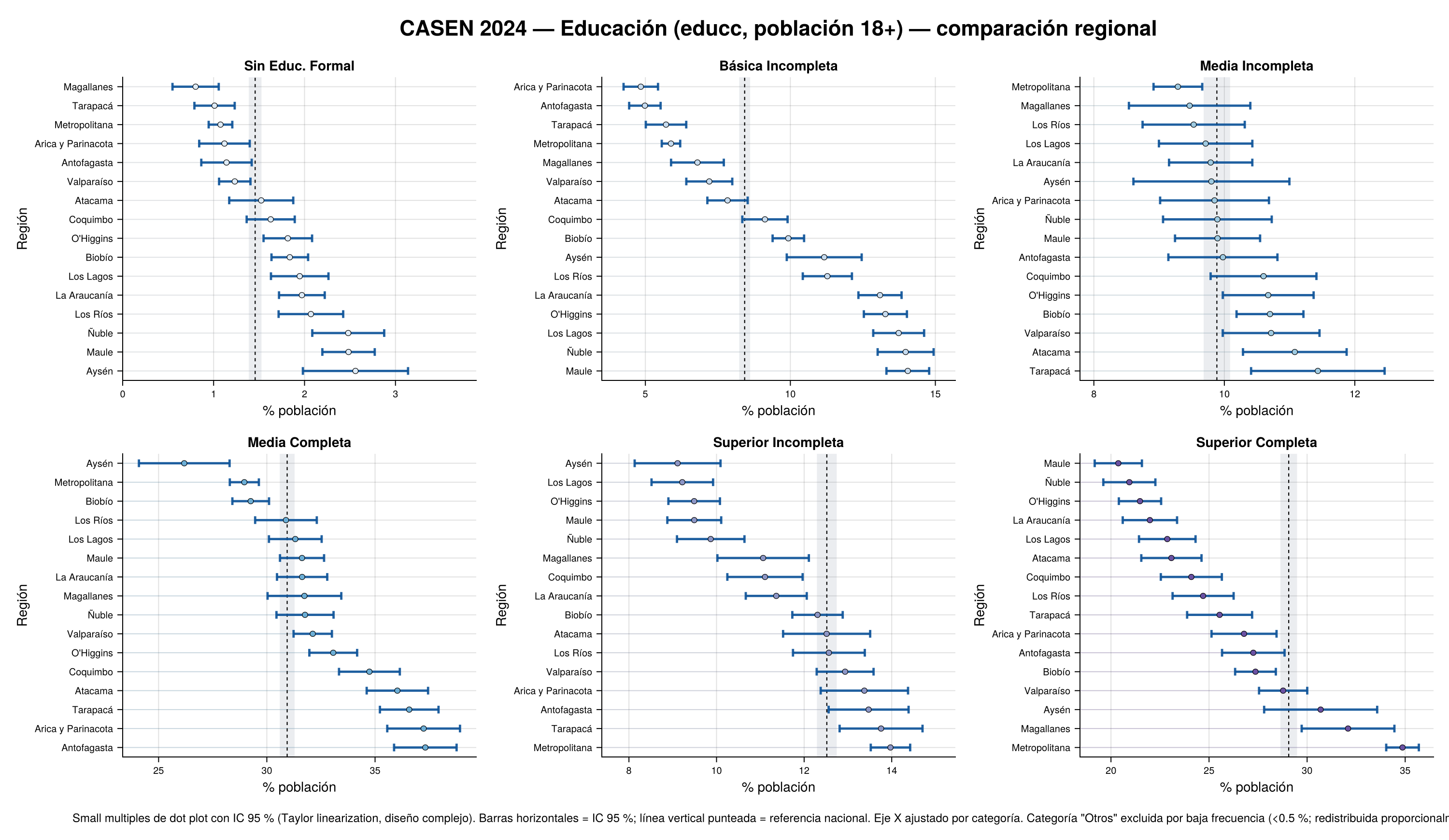
  <li><strong>Completed higher education</strong>: Metropolitana 34.9% [34.0%, 35.7%] versus Maule 20.4% [19.2%, 21.6%] — a gap of <strong>14.5 pp with non-overlapping CIs</strong>.</li>
</ul>

<p>The CIs are 95% and were computed by <strong>Taylor linearization</strong> (<a href="https://en.wikipedia.org/wiki/Linearization">wiki</a>) for CASEN’s complex sampling design (stratified two-stage, <code class="language-plaintext highlighter-rouge">expr</code> weights). That the CIs do not overlap implies these regional differences are statistically significant at the conventional level.</p>

<hr />

<h2 id="tolerance-to-contrast-or-checking-against-official-data">Tolerance to contrast, or checking against official data</h2>

<p>All results were checked against the official tables available in <a href="https://bidat.gob.cl/url/695ff7271b10e">BIDAT</a>.</p>

<p class="table-caption"><strong>Table 1</strong> — Official validation results (BIDAT, CASEN 2024)</p>

<table>
  <thead>
    <tr>
      <th>Parameter</th>
      <th>Value</th>
    </tr>
  </thead>
  <tbody>
    <tr>
      <td>Validation status (national + regional, % + expanded)</td>
      <td><strong>PASS</strong></td>
    </tr>
    <tr>
      <td>Maximum tolerance in percentage points</td>
      <td>1×10⁻⁵ pp</td>
    </tr>
    <tr>
      <td>Maximum tolerance in expanded values</td>
      <td>1×10⁻⁶</td>
    </tr>
    <tr>
      <td>Observed difference (pp)</td>
      <td>2.98×10⁻⁶ pp</td>
    </tr>
    <tr>
      <td>Observed difference (expanded)</td>
      <td>0.0</td>
    </tr>
    <tr>
      <td>National rows compared</td>
      <td>16</td>
    </tr>
    <tr>
      <td>Regional rows compared</td>
      <td>256</td>
    </tr>
  </tbody>
</table>

<p>The maximum observed difference is below 3 millionths of a percentage point, well within tolerance 😀. <strong>The results are numerically identical to the official ones.</strong></p>

<hr />

<h2 id="spoonful-1-sampling-design-and-expansion-without-shortcuts">Spoonful 1: sampling design and expansion without shortcuts</h2>

<p>CASEN 2024 has a <strong>probabilistic stratified two-stage</strong> design (<a href="https://bidat.gob.cl/url/69b71c77197db">BIDAT methodological note</a>). For regional-level estimates, the correct factor is <code class="language-plaintext highlighter-rouge">expr</code>; for the municipal level <code class="language-plaintext highlighter-rouge">expc</code> is required — they are not interchangeable. This analysis uses <code class="language-plaintext highlighter-rouge">expr</code> and reports estimates by region with 95% CIs computed by <strong>Taylor linearization</strong> over the complex design (strata, PSU/UPM and weights/factors).</p>

<p>Population represented in this run (sum of <code class="language-plaintext highlighter-rouge">expr</code>): <strong>20.13 million people</strong> (a pending task is to assess the impact of the new 2024 Census instead of projections over the 2017 Census).</p>

<div class="language-julia highlighter-rouge"><div class="highlight"><pre class="highlight"><code><span class="c"># CASEN 2024 sampling design specification</span>
<span class="n">design</span> <span class="o">=</span> <span class="x">(</span>
    <span class="n">weight</span> <span class="o">=</span> <span class="o">:</span><span class="n">expr</span><span class="x">,</span>     <span class="c"># regional expansion factor</span>
    <span class="n">strata</span> <span class="o">=</span> <span class="o">:</span><span class="n">estrato</span><span class="x">,</span>  <span class="c"># sampling stratum</span>
    <span class="n">psu</span>    <span class="o">=</span> <span class="o">:</span><span class="n">cod_upm</span><span class="x">,</span>  <span class="c"># primary sampling unit (PSU)</span>
    <span class="n">domain</span> <span class="o">=</span> <span class="o">:</span><span class="n">region</span><span class="x">,</span>   <span class="c"># estimation domain</span>
<span class="x">)</span>
</code></pre></div></div>

<p>Coverage by analyzed dimension:</p>

<p class="table-caption"><strong>Table 2</strong> — CASEN 2024 variables used and target population</p>

<table>
  <thead>
    <tr>
      <th>Dimension</th>
      <th>CASEN variable</th>
      <th>Target population</th>
    </tr>
  </thead>
  <tbody>
    <tr>
      <td>Education</td>
      <td><code class="language-plaintext highlighter-rouge">educc</code></td>
      <td>People ≥ 18 years</td>
    </tr>
    <tr>
      <td>Health</td>
      <td><code class="language-plaintext highlighter-rouge">s13</code></td>
      <td>Total population</td>
    </tr>
    <tr>
      <td>Poverty</td>
      <td><code class="language-plaintext highlighter-rouge">pobreza</code></td>
      <td>Total population</td>
    </tr>
  </tbody>
</table>

<h3 id="weighted-national-results">Weighted national results</h3>

<p>The following percentages correspond to proportions weighted with <code class="language-plaintext highlighter-rouge">expr</code>, validated against official data in BIDAT. The difference from the official values is &lt; 3×10⁻⁶ pp.</p>

<p class="table-caption"><strong>Table 3</strong> — Weighted national distribution (CASEN 2024, main categories)</p>

<table>
  <thead>
    <tr>
      <th>Dimension</th>
      <th>Category</th>
      <th style="text-align: center">% national</th>
    </tr>
  </thead>
  <tbody>
    <tr>
      <td>Education</td>
      <td>Complete secondary</td>
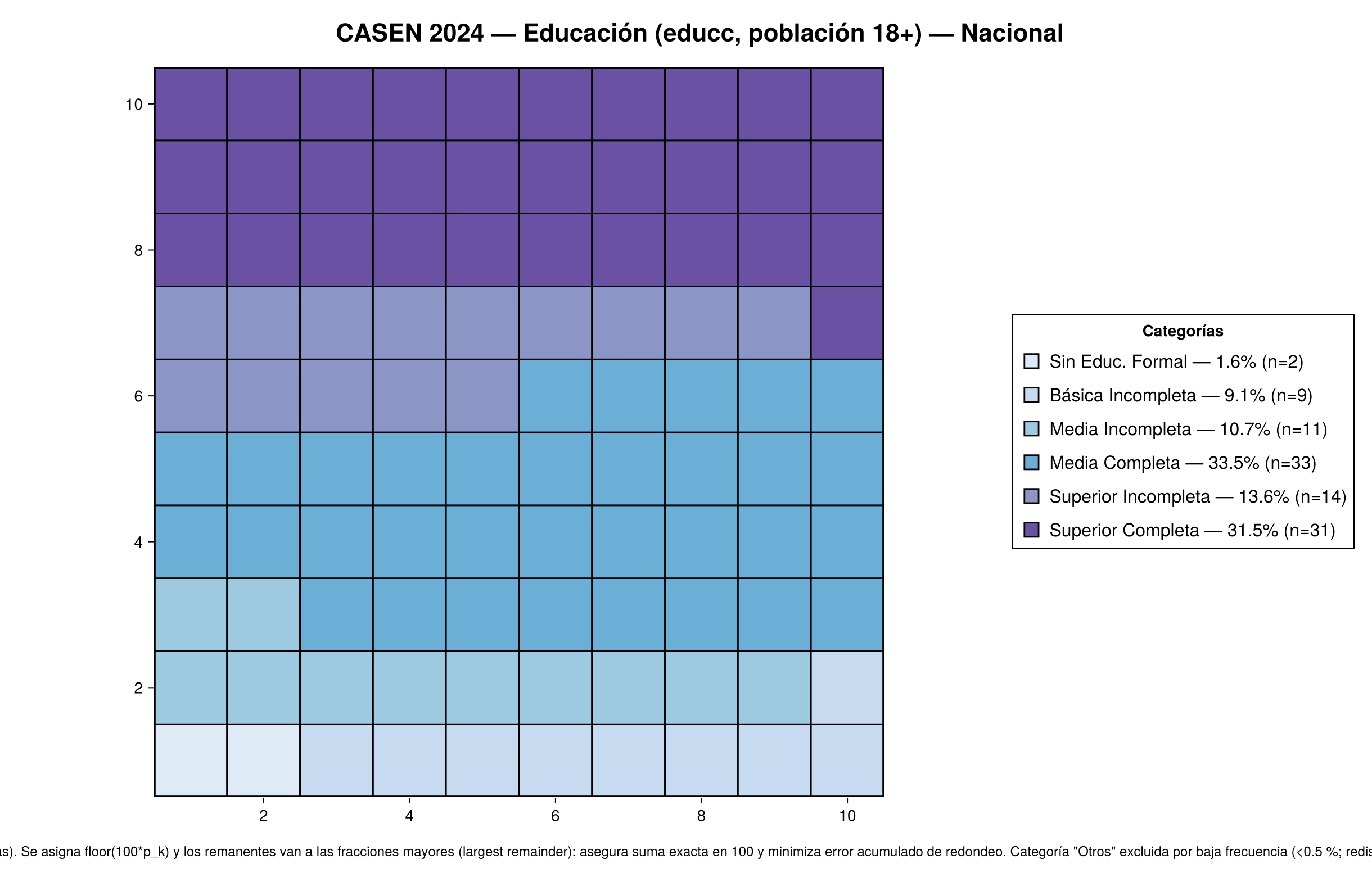
      <td style="text-align: center">30.9%</td>
    </tr>
    <tr>
      <td>Education</td>
      <td>Complete higher education</td>
      <td style="text-align: center">29.1%</td>
    </tr>
    <tr>
      <td>Education</td>
      <td>Incomplete higher education</td>
      <td style="text-align: center">12.5%</td>
    </tr>
    <tr>
      <td>Education</td>
      <td>Incomplete secondary</td>
      <td style="text-align: center">9.9%</td>
    </tr>
    <tr>
      <td>Education</td>
      <td>Incomplete primary</td>
      <td style="text-align: center">8.4%</td>
    </tr>
    <tr>
      <td>Education</td>
      <td>Other</td>
      <td style="text-align: center">7.7%</td>
    </tr>
    <tr>
      <td>Education</td>
      <td>No formal education</td>
      <td style="text-align: center">1.5%</td>
    </tr>
    <tr>
      <td>Health</td>
      <td>Public system FONASA</td>
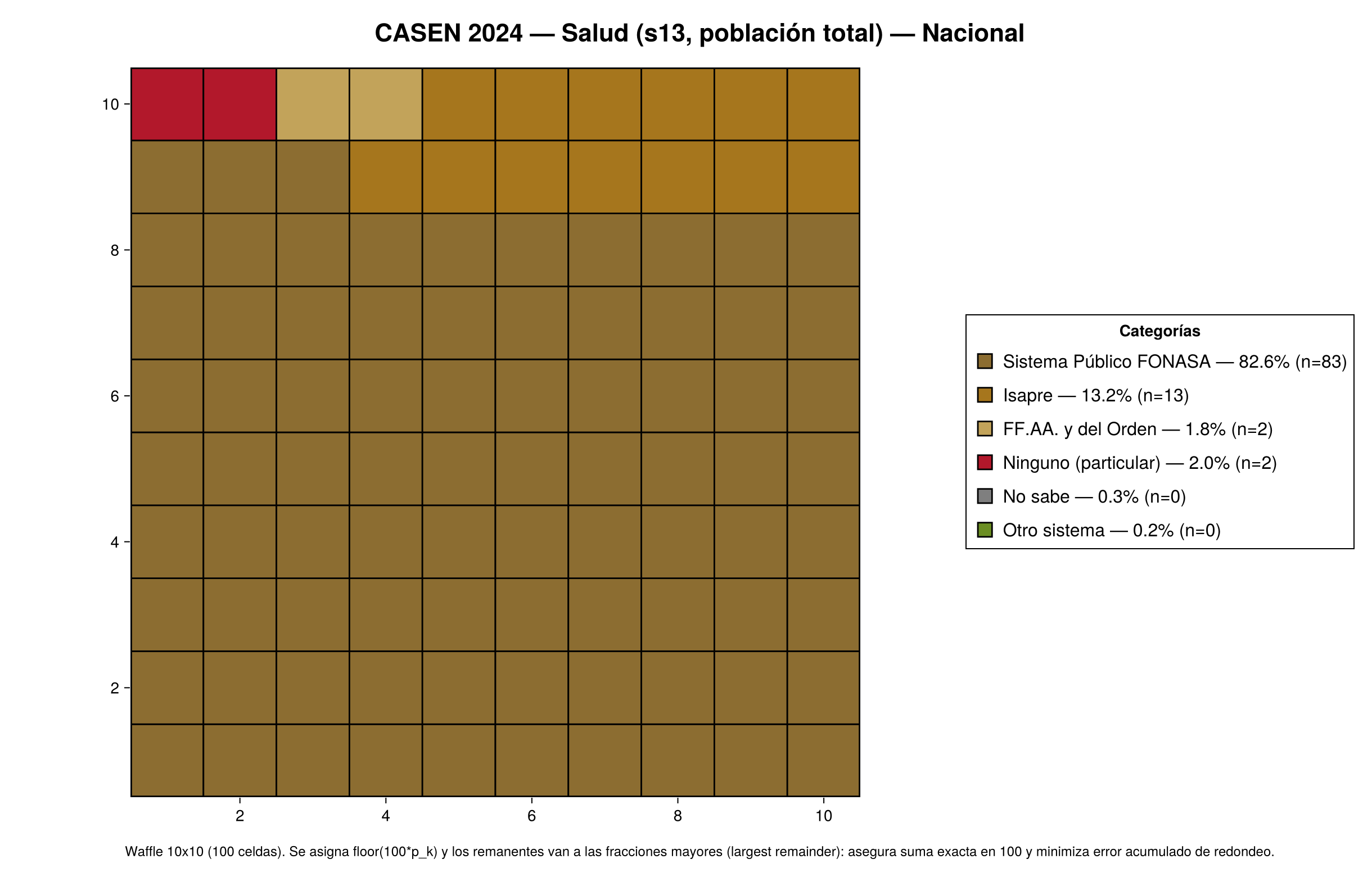
      <td style="text-align: center">82.6%</td>
    </tr>
    <tr>
      <td>Health</td>
      <td>Isapre</td>
      <td style="text-align: center">13.2%</td>
    </tr>
    <tr>
      <td>Health</td>
      <td>None (private out-of-pocket)</td>
      <td style="text-align: center">2.0%</td>
    </tr>
    <tr>
      <td>Health</td>
      <td>Armed forces and police</td>
      <td style="text-align: center">1.8%</td>
    </tr>
    <tr>
      <td>Health</td>
      <td>Does not know</td>
      <td style="text-align: center">0.3%</td>
    </tr>
    <tr>
      <td>Health</td>
      <td>Other system</td>
      <td style="text-align: center">0.2%</td>
    </tr>
    <tr>
      <td>Poverty</td>
      <td>Non-poverty</td>
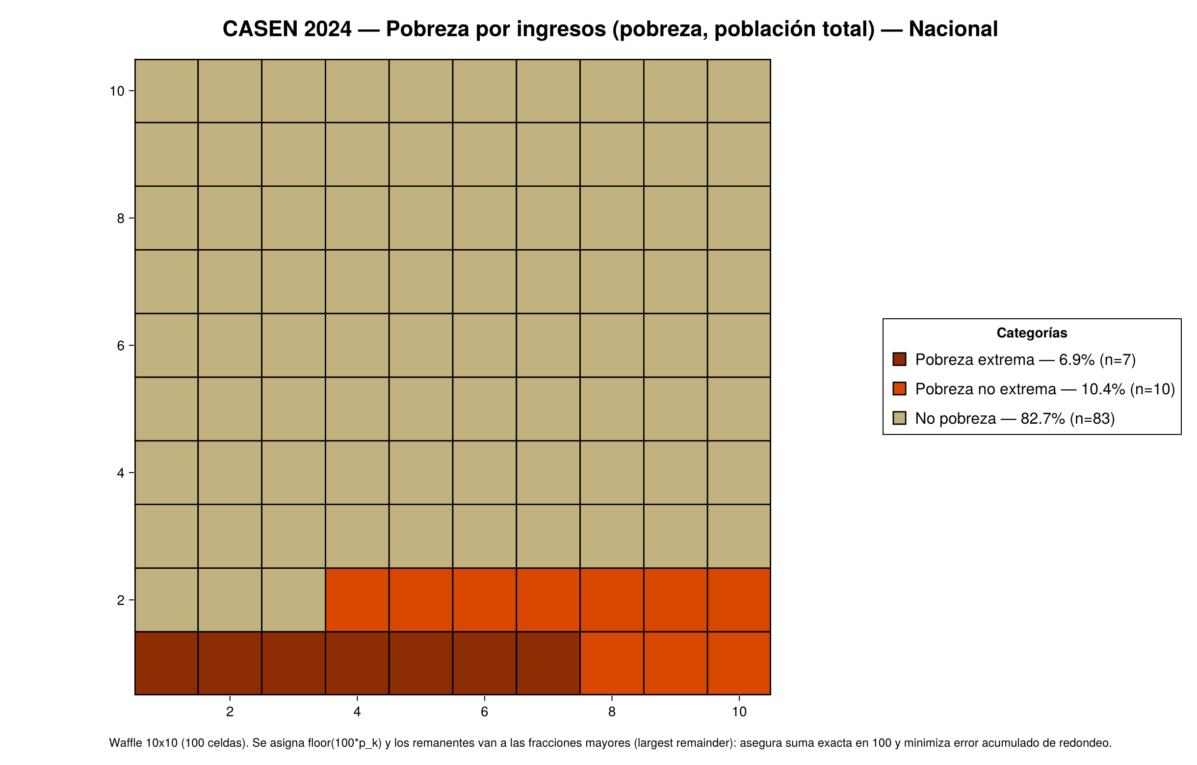
      <td style="text-align: center">82.7%</td>
    </tr>
    <tr>
      <td>Poverty</td>
      <td>Non-extreme poverty</td>
      <td style="text-align: center">10.4%</td>
    </tr>
    <tr>
      <td>Poverty</td>
      <td>Extreme poverty</td>
      <td style="text-align: center">6.9%</td>
    </tr>
  </tbody>
</table>

<hr />

<h2 id="spoonful-2-the-technical-flow-in-julia">Spoonful 2: the technical flow in Julia</h2>

<p>The pipeline runs end to end with <code class="language-plaintext highlighter-rouge">julia --project=. scripts/run_all.jl</code> (the orchestrator). The two most relevant pieces of code to reproduce and “audit” these results are the cell-allocation algorithm and the sampling-design specification (both in the GitLab/GitHub repository).</p>

<h3 id="taylor-linearization-se-and-ci-of-the-complex-design">Taylor linearization: SE and CI of the complex design</h3>

<p>A Taylor estimator was implemented for proportions in domains (regions). The linearized variable for the proportion $\hat{p}_d$ in domain $d$ is:</p>

\[z_j = \frac{1(j \in d)\,(1(\text{cat}_j = C) - \hat{p}_d)}{\hat{N}_d}\]

<p>The variance is estimated with the stratified cluster-design formula:</p>

<div class="language-julia highlighter-rouge"><div class="highlight"><pre class="highlight"><code><span class="c"># Taylor linearization variance (stratified, PSU)</span>
<span class="c"># e_{hi} = sum of w_j * z_j over PSU i in stratum h</span>
<span class="n">var_total</span> <span class="o">=</span> <span class="n">sum</span> <span class="n">over</span> <span class="n">strata</span> <span class="n">h</span><span class="o">:</span>
    <span class="x">(</span><span class="n">n_h</span> <span class="o">/</span> <span class="x">(</span><span class="n">n_h</span> <span class="o">-</span> <span class="mi">1</span><span class="x">))</span> <span class="o">*</span> <span class="n">sum_i</span> <span class="x">(</span><span class="n">e_</span><span class="x">{</span><span class="n">hi</span><span class="x">}</span> <span class="o">-</span> <span class="n">mean</span><span class="x">(</span><span class="n">e_h</span><span class="x">))</span><span class="o">^</span><span class="mi">2</span>

<span class="n">se</span>    <span class="o">=</span> <span class="n">sqrt</span><span class="x">(</span><span class="n">var_total</span><span class="x">)</span>
<span class="n">ci_lo</span> <span class="o">=</span> <span class="n">clamp</span><span class="x">(</span><span class="n">p̂</span> <span class="o">-</span> <span class="mf">1.96</span> <span class="o">*</span> <span class="n">se</span><span class="x">,</span> <span class="mf">0.0</span><span class="x">,</span> <span class="mf">1.0</span><span class="x">)</span>
<span class="n">ci_hi</span> <span class="o">=</span> <span class="n">clamp</span><span class="x">(</span><span class="n">p̂</span> <span class="o">+</span> <span class="mf">1.96</span> <span class="o">*</span> <span class="n">se</span><span class="x">,</span> <span class="mf">0.0</span><span class="x">,</span> <span class="mf">1.0</span><span class="x">)</span>
</code></pre></div></div>

<p>All PSUs of the design are used (including those outside the domain, with $z_j = 0$), which is correct for random-domain estimation. The median regional SE is <strong>1.66 pp</strong> of CI width; the maximum is <strong>5.76 pp</strong> (small regions with low-prevalence categories).</p>

<blockquote>
  <p><strong>Next entry, at some point 👀 — Jackknife and Bootstrap for CASEN as a contrast:</strong> TSL is an optimal first-order approximation for means and proportions, but for non-linear statistics (Gini, medians, quantile ratios) it can under-estimate the variance. The <a href="https://github.com/tatanlabra/casen24_julia_viz/blob/main/docs/ic-varianza-casen.md">code repository</a> includes the theory and the in-progress Julia code to contrast TSL with Jackknife (delete-1) and Bootstrap — a future entry in this series, which I have not reviewed in depth.</p>
</blockquote>

<h3 id="largest-remainder-why-it-matters-in-a-waffle-chart">Largest remainder: why it matters in a waffle chart</h3>

<p>A 100-cell waffle chart requires the proportions to add up to exactly 100 whole cells. Direct rounding introduces accumulated errors that make the sum 99 or 101. This flow uses the <strong>largest remainder</strong> algorithm, which guarantees the exact sum by introducing a slight imprecision for the sake of the visualization (take it as a purely visual nicety):</p>

<div class="language-julia highlighter-rouge"><div class="highlight"><pre class="highlight"><code><span class="s">"""
Allocate `n_cells` whole cells to proportions `p` using largest-remainder.
Guarantees that sum(cells) == n_cells exactly.
"""</span>
<span class="k">function</span><span class="nf"> allocate_cells</span><span class="x">(</span><span class="n">p</span><span class="o">::</span><span class="kt">AbstractVector</span><span class="x">{</span><span class="o">&lt;:</span><span class="kt">Real</span><span class="x">},</span> <span class="n">n_cells</span><span class="o">::</span><span class="kt">Int</span> <span class="o">=</span> <span class="mi">100</span><span class="x">)</span>
    <span class="n">raw</span>    <span class="o">=</span> <span class="n">p</span> <span class="o">.*</span> <span class="n">n_cells</span>
    <span class="n">floors</span> <span class="o">=</span> <span class="n">floor</span><span class="o">.</span><span class="x">(</span><span class="kt">Int</span><span class="x">,</span> <span class="n">raw</span><span class="x">)</span>
    <span class="n">remain</span> <span class="o">=</span> <span class="n">raw</span> <span class="o">.-</span> <span class="n">floors</span>
    <span class="n">deficit</span> <span class="o">=</span> <span class="n">n_cells</span> <span class="o">-</span> <span class="n">sum</span><span class="x">(</span><span class="n">floors</span><span class="x">)</span>
    <span class="c"># Assign remaining cells to the proportions with the largest remainder</span>
    <span class="n">idx</span> <span class="o">=</span> <span class="n">sortperm</span><span class="x">(</span><span class="n">remain</span><span class="x">,</span> <span class="n">rev</span><span class="o">=</span><span class="nb">true</span><span class="x">)[</span><span class="mi">1</span><span class="o">:</span><span class="n">deficit</span><span class="x">]</span>
    <span class="n">floors</span><span class="x">[</span><span class="n">idx</span><span class="x">]</span> <span class="o">.+=</span> <span class="mi">1</span>
    <span class="k">return</span> <span class="n">floors</span>
<span class="k">end</span>
</code></pre></div></div>

<p>Validated with unit tests: <code class="language-plaintext highlighter-rouge">allocate_cells([0.5, 0.3, 0.2], 100) == [50, 30, 20]</code>.</p>

<h3 id="reproducibility">Reproducibility</h3>

<div class="language-bash highlighter-rouge"><div class="highlight"><pre class="highlight"><code><span class="c"># Requirements: Julia 1.10+</span>
git clone &lt;repo&gt;
<span class="nb">cd </span>casen2024/julia_viz
julia <span class="nt">--project</span><span class="o">=</span><span class="nb">.</span> <span class="nt">-e</span> <span class="s2">"using Pkg; Pkg.instantiate()"</span>
julia <span class="nt">--project</span><span class="o">=</span><span class="nb">.</span> scripts/run_all.jl
</code></pre></div></div>

<p>The flow generates plenty of artifacts (CSV tables, PNG charts, audit logs for each input). The <code class="language-plaintext highlighter-rouge">Manifest.toml</code> file pins the exact versions of all dependencies (I used Julia 1.10).</p>

<hr />

<h2 id="spoonful-3-visual-evidence">Spoonful 3: visual evidence</h2>

<h3 id="national-composition-charts-13">National composition (Charts 1–3)</h3>

<p>Each waffle represents 100 cells allocated by largest remainder over the weighted proportions.</p>

<figure class="third ">
  
    
      <a href="/assets/images/casen2024-julia-waffles-politica-publica/waffle_educacion_educc.png" title="Chart 1 — Education: highest educational level attained (population ≥18 years, CASEN 2024)">
          <img src="/assets/images/casen2024-julia-waffles-politica-publica/waffle_educacion_educc.png" alt="Chart 1: Distribution of the highest educational level attained in the adult population (≥18 years), Chile, CASEN 2024. A 100-cell waffle chart with proportions by largest remainder." />
      </a>


      <a href="/assets/images/casen2024-julia-waffles-politica-publica/waffle_salud_s13.png" title="Chart 2 — Health: health insurance system (total population, CASEN 2024)">
          <img src="/assets/images/casen2024-julia-waffles-politica-publica/waffle_salud_s13.png" alt="Chart 2: Distribution of the health insurance system to which the population belongs, Chile, CASEN 2024. A waffle chart with 6 categories including FONASA, Isapre and others." />
      </a>


      <a href="/assets/images/casen2024-julia-waffles-politica-publica/waffle_trabajo_ingresos_pobreza.png" title="Chart 3 — Income poverty: extreme, non-extreme and non-poverty (total population, CASEN 2024)">
          <img src="/assets/images/casen2024-julia-waffles-politica-publica/waffle_trabajo_ingresos_pobreza.png" alt="Chart 3: Income poverty status in Chile according to CASEN 2024: extreme poverty, non-extreme poverty and non-poverty. A 100-cell waffle chart." />
      </a>


    <figcaption><strong>Charts 1–3</strong> — National composition: education (population ≥18 years), health and poverty (total population). Source: CASEN 2024, own elaboration in Julia. Values are validated against BIDAT. Click to enlarge.
</figcaption>
  
</figure>

<h3 id="regional-gaps-charts-46">Regional gaps (Charts 4–6)</h3>

<p>Each panel uses an <strong>axis fitted to the range of its own category</strong> (not a shared global scale), which makes it possible to visualize differences that flatten out if all categories share the same axis. The <strong>horizontal bars</strong> are 95% CIs computed by Taylor linearization. The hollow point (○) marks the national reference in each panel (with its CI).</p>

<figure class="third ">
  
    
      <a href="/assets/images/casen2024-julia-waffles-politica-publica/regional_dotplot_educacion_educc.png" title="Chart 4 — Regional gaps in education: dot plot by category (axis fitted per panel, hollow point = national reference)">
          <img src="/assets/images/casen2024-julia-waffles-politica-publica/regional_dotplot_educacion_educc.png" alt="Chart 4: Dot plot of regional gaps in educational level by category, CASEN 2024. Each panel has its axis fitted to its own range; a hollow point marks the national reference." />
      </a>


      <a href="/assets/images/casen2024-julia-waffles-politica-publica/regional_dotplot_salud_s13.png" title="Chart 5 — Regional gaps in health: dot plot by category (axis fitted per panel, hollow point = national reference)">
          <img src="/assets/images/casen2024-julia-waffles-politica-publica/regional_dotplot_salud_s13.png" alt="Chart 5: Dot plot of regional gaps in the health insurance system by category, CASEN 2024. Axis fitted per panel with national reference." />
      </a>


      <a href="/assets/images/casen2024-julia-waffles-politica-publica/regional_dotplot_trabajo_ingresos_pobreza.png" title="Chart 6 — Regional gaps in poverty: dot plot (axis fitted per panel, hollow point = national reference)">
          <img src="/assets/images/casen2024-julia-waffles-politica-publica/regional_dotplot_trabajo_ingresos_pobreza.png" alt="Chart 6: Dot plot of regional gaps in income poverty, CASEN 2024. Axis fitted per panel with national reference." />
      </a>


    <figcaption><strong>Charts 4–6</strong> — Regional gaps with 95% CIs (Taylor linearization, complex design): education, health and poverty. Bars = 95% CI; hollow point (○) = national reference. Axis fitted per category. Click to enlarge.
</figcaption>
  
</figure>

<h3 id="gaps-with-95-cis--all-statistically-robust">Gaps with 95% CIs — all statistically robust</h3>

<p class="table-caption"><strong>Table 4</strong> — Regional gaps with 95% CIs by Taylor linearization (CASEN 2024)</p>

<table>
  <thead>
    <tr>
      <th>Dimension</th>
      <th>Category</th>
      <th style="text-align: center">Gap (pp)</th>
      <th>Maximum</th>
      <th>95% CI</th>
      <th>Minimum</th>
      <th>95% CI</th>
    </tr>
  </thead>
  <tbody>
    <tr>
      <td>Poverty</td>
      <td>Non-poverty</td>
      <td style="text-align: center"><strong>18.6 pp</strong></td>
      <td>Magallanes 90.0%</td>
      <td>[88.5%, 91.5%]</td>
      <td>La Araucanía 71.4%</td>
      <td>[69.8%, 73.0%]</td>
    </tr>
    <tr>
      <td>Health</td>
      <td>Isapre</td>
      <td style="text-align: center"><strong>16.3 pp</strong></td>
      <td>Metropolitana 20.6%</td>
      <td>[19.8%, 21.5%]</td>
      <td>Maule 4.3%</td>
      <td>[3.7%, 5.0%]</td>
    </tr>
    <tr>
      <td>Health</td>
      <td>FONASA</td>
      <td style="text-align: center"><strong>15.2 pp</strong></td>
      <td>La Araucanía 91.1%</td>
      <td>[90.2%, 92.0%]</td>
      <td>Metropolitana 75.9%</td>
      <td>[75.0%, 76.7%]</td>
    </tr>
    <tr>
      <td>Education</td>
      <td>Complete higher education</td>
      <td style="text-align: center"><strong>14.5 pp</strong></td>
      <td>Metropolitana 34.9%</td>
      <td>[34.0%, 35.7%]</td>
      <td>Maule 20.4%</td>
      <td>[19.2%, 21.6%]</td>
    </tr>
    <tr>
      <td>Poverty</td>
      <td>Extreme poverty</td>
      <td style="text-align: center"><strong>8.8 pp</strong></td>
      <td>La Araucanía 13.0%</td>
      <td>[11.8%, 14.1%]</td>
      <td>Magallanes 4.2%</td>
      <td>[3.1%, 5.2%]</td>
    </tr>
  </tbody>
</table>

<p>In every case the CIs do not overlap: the gaps are statistically significant at 5%. CIs computed by Taylor linearization over the complex design (strata, PSU/UPM, <code class="language-plaintext highlighter-rouge">expr</code>).</p>

<hr />

<h2 id="closing-three-questions-for-those-who-use-the-survey">Closing: three questions for those who use the survey</h2>

<p>If you use CASEN 2024 for territorial characterization or other uses where regional-level variables matter, think twice before using a point estimate (without its confidence interval):</p>

<ol>
  <li><strong>Are your results validated against BIDAT and do they carry design-based CIs?</strong> A difference greater than 1×10⁻⁵ pp from the official tables is not technical: it is a process issue. And without complex-design CIs, an 8 pp gap can look like evidence when it is noise in small regions.</li>
  <li><strong>Are you using the correct expansion factor?</strong> <code class="language-plaintext highlighter-rouge">expr</code> is the right one for regions; <code class="language-plaintext highlighter-rouge">expc</code> for municipalities. They are not interchangeable, and using the wrong one biases coverage estimates.</li>
  <li><strong>Is your analysis reproducible?</strong> A flow that cannot be audited cannot be defended before a technical counterpart, nor updated when CASEN 2026 is released.</li>
</ol>

<p>The CIs incorporated here are complex-design (Taylor linearization), not simple asymptotic ones. They cover sampling variance but not non-response error or undercoverage. Causal inference between subpopulations requires additional design.</p>]]></content><author><name>Cristián Labra Olivares</name></author><category term="datos" /><category term="politica-publica" /><category term="julia" /><category term="casen" /><category term="casen2024" /><category term="julia" /><category term="expansion" /><category term="sampling-design" /><category term="waffle" /><category term="dotplot" /><category term="public-policy" /><category term="bidat" /><category term="territorial-gap" /><summary type="html"><![CDATA[A reproducible analysis of CASEN 2024 in Julia: official validation against BIDAT data, national composition via waffle charts, and regional gaps in education, health and poverty for territorial prioritization.]]></summary></entry></feed>